Single dataset analysis

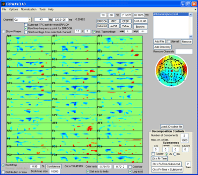
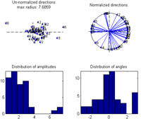
Once the generated file is loaded the currently selected measure is calculated and displayed in the montage plot. By left clicking the mouse over the montage plot each channel-time-frequency point can be inspected. Click on a point and select:

Tools -> Show distribution of complex coefficients through the epochs at current point

a plot giving the complex coefficient at each epoch is given (right plot below) along with the distribution of amplitudes lower left and angle lower right.

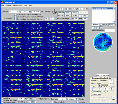
Note: All the measures can be decomposed in this way. The lower level of the color axis is subtracted before decomposing such that only regions currently above this threshold is decomposed.

Select ‘Incl. Topmontage’ to get the activity in each channel at their specified location. Select ‘Rayleigh distribution’ and press the ‘Confidence’ button. Regions that are less likely by a  5 % confidence to occur by random are marked by red contours.  Select the ‘distribution of max’ so that the confidence is corrected for multiple comparison treating each channel-time-frequency point as a separate independent observation. Currently, there are not enough epochs in the dataset to establish any significant regions using ‘distribution of max’.

Select Normalization -> Pre Normalization -> Normalize by baseline activity

And specify the baseline region to be for instance from –101.6 ms to –7.8 ms.

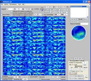
Click the ‘Confidence’ button such that confidences are no longer calculated. Deselect the ‘Log-axis’ and Press the ITPC button to display the ITPC. Click in the montage plot on a region with strong ITPC activity.  Press the ERPCOH button. The cross coherence from the point currently selected to all other points is calculated and displayed in the montage plot.

In bold above the details of the currently selected point is displayed the selected point from which the ERPCOH was calculated.

Select another point in the montage plot. The cross coherence from the point previously selected to the point selected is then given. Select:

Cross View -> Record cross coherence

This coherence is now recorded for plotting. Click the ERPCOH button and calculate the cross coherence to all other points from this newly selected point.  Select a new point and record this point by:

Cross View ->Record cross coherence.

To display the recorded cross coherences select:

Cross View -> View recorded cross coherences.

A plot of each recorded coherence is given as well as a summary plot of all coherences. The relative strength of the coherences is given as the color of the arrows (light gray indicates week activity compared to black arrows). Each individual plot specifies the details of the coherence recorded including the probability of the coherence to occur by random with the found strength (if ‘distribution of max’ is selected this value is corrected for multiple comparison)

Click the ‘Remove’ button just below the file browser. You are now ready to continue to multiple dataset analysis.

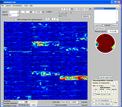
Since no epochs have been rejected, we first inspect the epochs for artifacts. Press the ‘Epochs button’.

Press the ‘abs(STD)’ button to inspect the absolute value of the standard deviation of the amplitudes of each epoch to the mean value over all epochs. Set the array of the montage plot to 16 x 3 instead of 16 x 4. Reject epoch 14, 32 and 36 by specifying these epochs in the area above the channel map. Press the ‘Epochs’ button again to reject the marked epochs.  Press ‘Yes’ when asked to reject the marked epochs and save the new dataset.

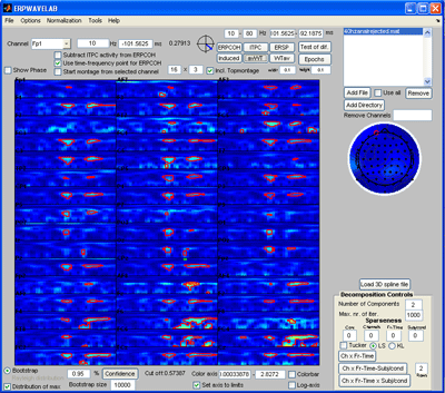
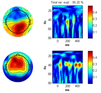
Press the ‘ITPC’ button to inspect this measure again (note, whereas the other measures are strongly influenced by noisy epochs the ITPC gives the same weight to each epoch . Thus, noisy epochs have little influence on this measure.). Set the sparseness on the Fr-Time to 0.1 and press the ‘Ch x Fr –Time’ button. A two component model of the ITPC activity is fitted given to the right below. Press ‘Cancel’ in the window that opens asking you to save the decomposition results if you don’t want to save these.

Select Normalization -> Post normalization ->  Normalize by background activity.

Each measure is now normalized by its baseline value. Deselect ‘distribution of max’ and click the ‘Induced’ button. Furthermore, select log-axis. The significant regions of the induced activity compared to baseline is now given as blue (reduced) regions and red (increased) regions.

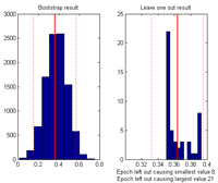
By selecting:

Tools -> Show distribution of current measure at currently inspected point

a plot giving the distribution of the current value at the selected channel-time-frequency is given. Left plot by bootstrapping, right plot by leave one epoch out at a time.

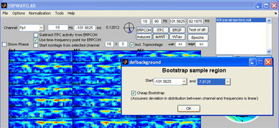
Press the ‘avWT’ button. Since the confidence button is pressed a two tailed 95 % confidence interval is calculated by bootstrapping. Select the bootstrap sample region to be the same as the baseline region. The ‘Cheap bootstrap’  normalizes each channel and frequency point, calculates one bootstrap sample using these normalized values and multiplies the sample distribution by the normalization factor found for each channel and frequency. This is significantly faster than calculating separate bootstrap samples for each channel and frequency, however, it assumes the deviation between distribution of each channel frequency region is a simple multiplication by a constant. If this is not selected, the full bootstrap over all channels and frequencies is calculated. Red contours are regions significantly elevated, green contours are regions significantly reduced (note: Calculating the contours can take a long time).

Developed by Morten Mørup

A tOOLbox FOR MULTI-CHANNEL TIME-FREQUENCY ANALYSIS