Multiple dataset analysis

Download tutorial dataset 2 and un-zip the files containing the ITPC-ERPWAVELAB files of 14 subjects during right and left hand stimulation (a total of 28 datasets) . Click the

‘Add Directory’ button and select the folder containing the unzipped files.

If the ‘Statistics Toolbox’ of MATLAB is installed click Tools ->Dendrogram.

A dendrogram clustering the datasets according to their Euclidian distances in the channel-time-frequency plot of the current measure (here the ITPC) is given. (This takes a while, go to the MATLAB prompt to follow the progress)

Click the ‘Test of dif.’ button, a window opens to select groups. There are two group present in the data, left hand stimulation (dataset starting with L) and right hand stimulation dataset starting with (R). 

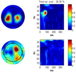
Once all datasets corresponding to left has been set to Group 1 and all datasets corresponding to right to Group 2 click ‘Done’. The F-test value of Analysis of Variance (ANOVA) between group means at each channel-time-frequency point is displayed in the montage plot. Only activities significant elevated by a 95 % confidence is displayed. No F-test value is this significant. Instead, click the ‘Set axis to limits’ to display all the F-test values. Set the ‘time-frequency’ sparseness to 0.1 and click the ‘Ch x Fr-Time’ button. The ANOVA F-test array is decomposed giving a two component model similar to the one shown to the right below revealing that the major difference between the two groups are in the central left and right regions of the scalp at 30-40 Hz 80 ms.

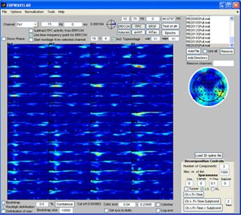
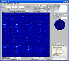
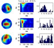
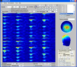
Click on one of the files in the ‘file browser’ or click the ‘ITPC’ button to again display the ITPC of the currently selected file. To not display the theoretical background ITPC activity set the confidence level to 0.5 and press the ‘Confidence’ button. Read of what the theoretical cut off (background activity is) and enter it as the lower limit to the color axis.

Set sparseness to 0.1 for time-frequency, set the number of components to 3 and click the ‘Ch x Fr-tim-subj/cond’ a decomposition of the datasets finding the scalp regions of most similar activity over the subjects but varying in time-frequency signature will be given. Once this decomposition has been found click the ‘Ch x Fr-time x subj/cond’ button. The activity the most similar in channels and in the time-frequency domain over the dataset will be found as well as the strength in which this activity is present in each dataset, see figures below.

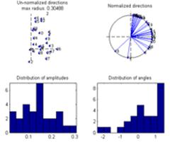
Finally, click the ’Use all’ checkbox. The grand average of the current measure (presently the  ITPC) of all datasets is calculated and displayed in the montage plot. Select

Options -> Show distribution of complex coefficients through the epochs at current point

Where previously the distribution over epochs was displayed, now that ‘Use all’ is selected, the distribution over datasets is instead given, see lower right figure.

You’ve now completed the tutorial showing the most commonly used functionalities of ERPWAVELAB. For a full description of all functions consult the ERPWAVELAB HELP.

If you want the channel activity to be displayed as 3D head plots, click the ‘Load 3D spline file’ below the channel activation plot. Go to the ERPWAVELAB subfolder ‘Splines’ and open the ‘3D-64CHANNEL’ spline file.

By selecting:

Tools -> Show distribution of current measure at currently inspected point

a plot giving the distribution of the current value at the selected channel-time-frequency is given. Left plot by bootstrapping over the datasets, right plot by ‘leave one dataset out’ at a time.

Developed by Morten Mørup

A tOOLbox FOR MULTI-CHANNEL TIME-FREQUENCY ANALYSIS